이번에는 MAR 두번째 논문이다. MAR 연구 특성상 사람한테 한번 metal을 박으면 metal이 없는 CT를 얻을 수가 없기 때문에 data 부족 문제에 시달릴수밖에 없고, 이것을 해결하기 위해 나는 data synthesize 방법을 취했지만, unsupervised로는 어떻게 푸는지 궁금해서 논문을 읽어보았다!
unsupervised i2i에서 가장 베이스로 사용되는 cycleGAN에서 발생하는 문제인 input domain 생성은 잘 되지만 target domain 생성이 잘 안되는 문제가 여기서도 발생했었는지, 발생했다면 그걸 해결하려고 했는지가 궁금했다. (다 읽고 나니 그게 β-CycleGAN인 이유인것 같다)
Introduction
- FDK(Feldkamp, Davis and Kress) is the most widely used algorithm
- metal implants 삽입이 ROI부근에 일어나면서 MAR이 중요해졌다
- X-ray photons cannot penetrate the metallic object consistently due to the object’s high attenuation
- this causes severe streaking and shading artifacts that deteriorate the image quality in reconstructed images
Related Works
Conventional Methods
modify the sinogram and recnstruct objects by removing the corrupted sinogram and interpolating it from adjacent data
Conventional method들은 대부분 사이노그램단에서 이루어지는데, metal artifact 부분을 마스킹하고 주변 픽셀 값으로 마스크를 interpolation하는 방법이 주를 이룬다.
- LI-MAR
- replaces the metallic parts in the original sinogram with linear interpolated values from the boundaries
- this usually causes new artifacts due to inaccurate values interpolated in the metallic parts in the sinogram
- NMAR
- sinogram의 normalized 값을 이용하여 interpolation
- still have a limitation for generate applications due to the difficulty of optimal parameter selection
⇒ difficulty of optimal parameter selection (결국 rule-based가 아니라 optimal한 파라미터를 찾는 deep learning을 사용하겠다는 말이다.)
- iterative reconstruction methods (iMAR)
- iterative하게 CT reconstruction을 하게 되면 artifact가 사라진다는 연구가 있었지만, 경험상 artifact를 완벽하게 지우지는 못하고 이런 효과가 있네?의 느낌이다.
- 그리고 당연하겠지만 extremely high computational complexity
DL-based Methods (supervised)
- CNN based, pix2pix
- sinogram network and the image network by learning two CNNs (dudonet)
⇒ all supervised methods
⇒ to utilize pairs of unmatched images, unsupervised learning approaches should be used.
GAN이 input domain의 distribution에서 target domain distribution을 잘 match 시킬 수 있다
그러나 GAN 자체로는 mode collapse 문제가 존재하므로, cycle-consistent adversairal network
- Recently, the mathematical origin of cycleGAN was revealed using optimal transport theory as an unsupervised distribution matching between two probability spaces.
Unsupervised MAR Methods
- ADN
- artifact disentanglement network
- ADN은 artifact-affected image에서 artifact와 content components를 각각 encoding 하여 각각의 공간으로 보냄으로써 분리시키는 방법
- disentangle이 잘 되었다면 content component가 content information은 모두 가지고 있으면서 artifact에 대한 정보는 하나도 가지고 있지 않을 것
- 안좋은점
- highly complicated network architecture due to the explicit disentanglement steps.
- training에 등장하지 않은 artifact에 대해서는 artificial feature가 나타남
- 그리 효과적이지는 않은 것 같고, artifact를 disentangle하겠다는 관점으로 접근했다는 점이 contribution인 것 같다. 그리고 disentangle을 하려고 모델 구조가 되게 복잡해져버리는 단점이 있다.
- method proposed by Ranzini et al.
- uses paired MRI and CT
β-VAE for feature space disentaglement
논문이 β-VAE에서 아이디어를 얻어서 만들어졌기 때문에, β-VAE에 대한 기본을 공부해보자.
maximize ELBO! \(p_\theta(x|z)\) : decoder (z→x) ..\(q_\phi(z|x)\) : encoder (x→z) \(q_\phi(z|x)\) : user-chosen posterior distribution model parameterized by \(\phi\).
objective function: ㄴ \(logp_{\theta}(x) = log(\int p_{\theta}(x|z)p(z)dz)= log(\int p_{\theta}(x|z){p(z) \over q_\phi(z|x)}q_\phi(z|x)dz)\)
Jensen’s Inequality에 의해,
\[log(\int p_{\theta}(x|z){p(z) \over q_\phi(z|x)}\;q_\phi(z|x)dz) >= \int log({p_\theta(x|z)p(z) \over q_\phi(z|x)})\;q_\phi(z|x)dz\]얘는 이렇게 두개로 가를 수 있고,
\[\int log({p_\theta(x|z)p(z) \over q_\phi(z|x)})\;q_\phi(z|x)dz = \int log(p_\theta(x|z))q_\phi(z|x)dz + \int log({p(z)\over q_\phi(z|x)})q_\phi(z|x)dz\]KL-divergence를 활용하기 위해 이 식을 보자.
Kullback–Leibler divergence
\[D_{KL}(P||Q)=\int_{\infty} p(x)log{p(x) \over q(x)}dx\]이것을 적용하면,
\[\int log({p(z)\over q_\phi(z|x)})q_\phi(z|x)dz = -\int log({q_\phi(z|x)\over p(z)})q_\phi(z|x)dz = -D_{KL}(q_\phi(z|x)||p(z))\]결국
\[logp_{\theta}(x) >= \int log\, p_\theta(x|z) q_\phi(z|x)dz - D_{kl}(q_\phi(z|x)||p(z))\] \[- logp_{\theta}(x) <= - \int log\, p_\theta(x|z) q_\phi(z|x)dz + D_{kl}(q_\phi(z|x)||p(z))\]그런데 KL divergence의 최솟값이 0이므로 upper bound의 minimize가 가능해진다.
이렇게 유도된 VAE 식의 KL-divergence에 $\beta$를 붙인 걸 $\beta$-VAE라고 부른다. 베타를 붙인 이유는
- As a high $\beta$ imposes more constraint on the latent space, it turns out that the latent space is more interpretable and controllable, which is known as the disentanglement.
- $\beta$가 작을수록 z에 constraint를 줄이는 효과가 나서 표현력이 커지고, 클수록 z가 하나의 가우시안에 근사되어 표현력이 낮아짐(VAE는 분포를 가우시안에 근사하므로)
level of feature disentanglement
- inspired by β-VAE(vairaitonal uatoencoder), we control the level of the importance in terms olf the statistical distances in the original and target domains using a weighting parameter β.
- $\beta$-VAE처럼 cycleGAN에서 weighting paramter β를 활용해 학습을 조절하겠다는 게 이 논문의 의의이다!
Theory
-
the transportation from a measure space (Y,ν) to another measure space (X, $\mu$)
$G_\theta : Y -> X$
- the transportation from (X, $\mu$) to (Y, v) : $F_\phi : X->Y$
- Unsupervised learning에서 optimal transport map은 dist($\mu_\theta, \mu$)와 dist($v_\phi, v$)를 minimize하는 것으로 얻을 수 있다
각각을 따로 minimize하는 대신, joint distribution $\pi$에 대해 같이 minimize
\[inf \int ||x-G(y)|| + ||F(x)-y|| d\pi(x,y)\]“Optimal transport, cycleGAN, and penalized LS for unsupervised learning in verse problems” 논문에서 위 식을 dual formulation으로 나타낼 수 있다고 함.
\[min_{\theta, \phi} max \; l_{cycleGAN}(\theta, \phi, \psi, \varphi) := \lambda l_{cycle}(\theta, \phi) + l_{Disc}(\theta, \phi; \psi, \varphi)\] \[l_{cycle}(\theta, \phi) = \int_X ||x-G_\theta(F_\phi(x))||d\mu(x) + \int_Y||y-F_\phi(G_\theta(y))||dv(y)\] \[l_{Disc}(\theta, \phi; \psi, \varphi) = max \int_{X}D_\psi (x) d\mu(x)-\int_Y D_\varphi(G_\theta(y))dv(y) + max \int_{Y}D_\psi (y) dv(y)-\int_Y D_\varphi(F_\phi(x))d\mu(x)\]- 따라서 이 form은 1-Lipschitz discriminators를 사용한 것만 빼면 기존 cyclegan과 동일하다.
- LS-GAN 방법론이 imposing the finite Lipschitz condition과 깊은 관련이 있다는 것을 보임
- LS-GAN variation as our discriminator term을 사용
$\beta$-CycleGAN for metal artifact disentanglement
- VAE처럼 G와 F에 다른 weight를 주겠다는 게 point이다. (실제로 cycleGAN 실험을 해 보면 G는 잘되는데 F는 안되고 이런 문제가 있다)
Y에서Metal artifact 정도가 모두 다르고, 심지어 clean 이미지도 가지고 있는 경우도 있음- 따라서 clean(CT without metal artifact)은 input과 동일한 output을 내놓아야 하므로 Identity loss를 사용
최종 objective:
\[l_{MAR}(\theta, \phi; \psi, \varphi) := l_{\beta-cycle}(\theta, \phi) + l_{Disc}(\theta, \phi; \psi, \varphi)+\gamma l_{identity}(\theta, \phi)\]Geometry of Attention
-
artifact가 발생할 수 있는 부분과, 그 부분에 집중할 수 있게 해주는 모듈을 도입
- To address these issues, a method mimicking the human visual system can be a good option because humans exploit a sequence of partial glimpses and selectively focus on salient parts in order to capture the visual structure much better.
-
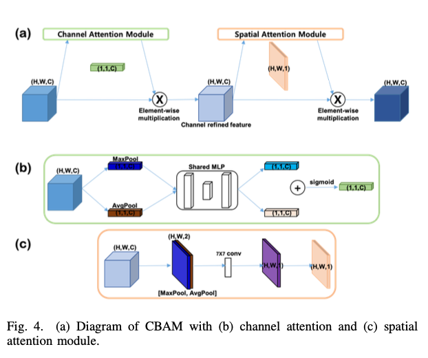
The convolutional block attention module(CBAM) is one of the simplest yet effective one.
- GAN-based deep convolutional networks는 geometric/structural pattern을 잘 못 잡아냄
- due to small receptive field from convolution operator
- kernel size를 키우면 되긴 하지만 computational and the statistical efficiency가 작아짐
- global dependencies를 잡는 attention mechanisms
- self attention
- SAGAN efficiently learns to find global and long-range of dependencies within internal representationss of images
- 그러나 calculating the key and query from entire images is often computationally expensive and can cause memory problems as the spatial sizes of input get bigger
- CBAM
- simple yet effective
- self attention
- 여기서는 self-attention 대신 CBAM 모듈을 사용했는데, 역시 동감한다. self-attention은 너무 무겁고 생각만큼 안 좋은데, CBAM을 쓰면 훨씬 가벼우면서 성능도 잘 나온다. (나도 처음에 CBAM 사용을 고려했다)
A: spatial attention map, T: channel attention map, Z: feature map
- Deep convolutional framelets theory에 의해, 이것은 1x1 conv 후 global pooling을 하는 것과 동일
- CBAM은 spatial/channel attention을 모두 유지하면서, computational complexity도 작게 가져가는 좋은 attention model
- Channel attention module
- Channel attention focuses on ‘what’ are important channels
- layers
- average pooling : aggregate spatial information (squeeze)
- maxpooling : gathering another iportant clue about distinctive object features
- two multi-layer perceptron (squeeze)
- Spatial attention module
- focuses on ‘where’ is an informative
- average pooling & maxpooling used
- 7x7 convolution operator
저 channelwise attention이랑 spatial attention을 같이 쓰는 방법론이 되게 많이 나왔는데, CBAM은 channel attention과 spatial attention을 따로 태운 후 merge하는 형태가 아니라 순차적으로 channel attention, spatial attention을 태우기 때문에 가볍다. (개인적으로는 그래서 더 안정적인 것 같기도 하다..?)
Meterials and Methods
Dataset
- Real Metal Artifact Data
- From the equal-spaced conebeam projection data, we reconstructed the CT images by FDK.
- 504x504x400
- 3 patients for training, 1 patients for validation, 1 patients for test
- 800 with metal artifact 400 without metal artifacts
- Synthetic Metal Artifact Data
- 10997 artifact-free images for LiTS (Liver Tumor Segmentation Challenge)
- CNN-MAR과 동일한 방법론으로 synthesize
- simulates the beam hardening effect and Poisson noise
- 5860 artifact 4115 clean for train
- 373 artifact 335 clean for test
- 256x256 (비교실험 때 ADN이 너무 커서 512x512 할수 없었음)
Network Architecture
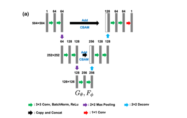
- $G_\theta, F_\phi$ 모두 U-net + attention in skip/concatentation 으로 진행된다. MAR을 해본 경험으로써 저 skip쪽에 attention 모듈을 다는 게 되게 중요한데, 그 이유가 encoder feature에서 미처 제거되지 못한 artifact들이 이후에 decoder와 concat하면서 다 살아나 버리기 때문에, encoder feature에 attention을 붙여 artifact를 떨어뜨려 가면서 concat하는 게 매우 관건이다. 여기도 그걸 알고 네트워크를 이런 식으로 구성한 것 같다.
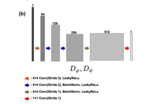
- $D_\psi, D_\varphi$ 는 PatchGAN base 4 conv + fc with batchnorm
Training Detail
- input : 504 x 504
- $\lambda = 10, \beta = 1, \gamma=1$
- $\beta$가 클수록 모델이 artifact-free image generation에 집중하는 경향을 보임
- useful in real data case
- metal artifact가 없는 이미지라도 beam hardening artifacts가 있을 수 있기 때문에 identity loss를줌
- lessening the value of the hyper-parameter that is involving property that do not need to be changed
- 50 epoch (early stopping)
- xavier initializer
-
lr : 2x10⁻³
- synthetic data에서
- 256x256
- $\lambda = 10, \beta = 1, \gamma=5$
- synthetic data는 artifact generation procedure가 simple하기때문에, two statistical distance에 동일한 weight를 사용
- no artifacts in the images with no metal artifacts, 따라서 높은 identity loss rate
Real data
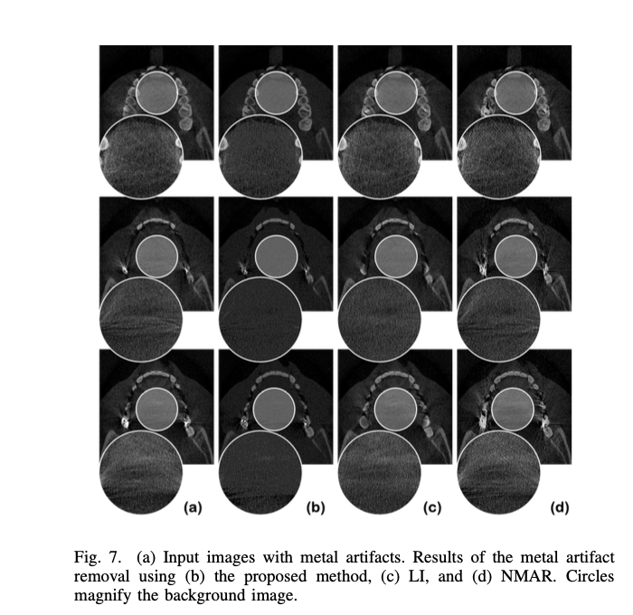
(a) input (b) proposed (c) LI (d) NMAR (e) ADN with downsampled input (f) proposed with downsampled input
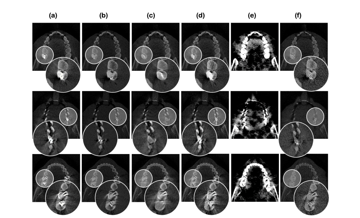
Homogeneous region (tissue)
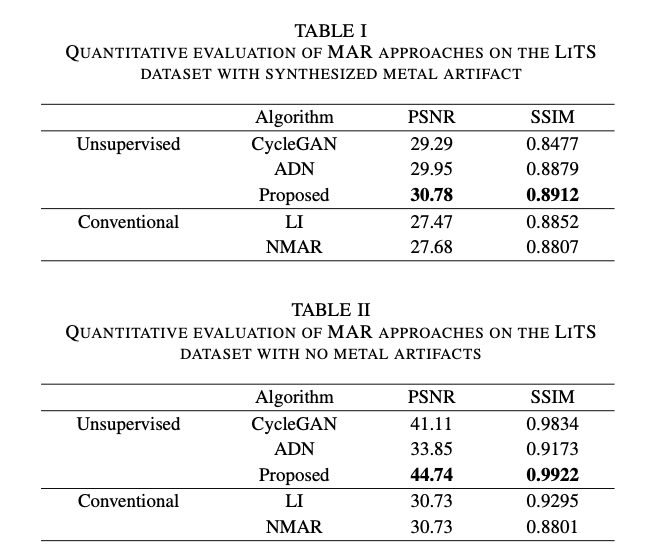
아쉬운 점은 supervised 방법론과의 비교는 없다는 점이다. 아무래도 synthetic data가 어느 정도 realistic할 수 있는 metal artifact reduction에서 self-supervised가 supervised를 이기기에는 무리가 있었지 않나.. 생각이 든다.
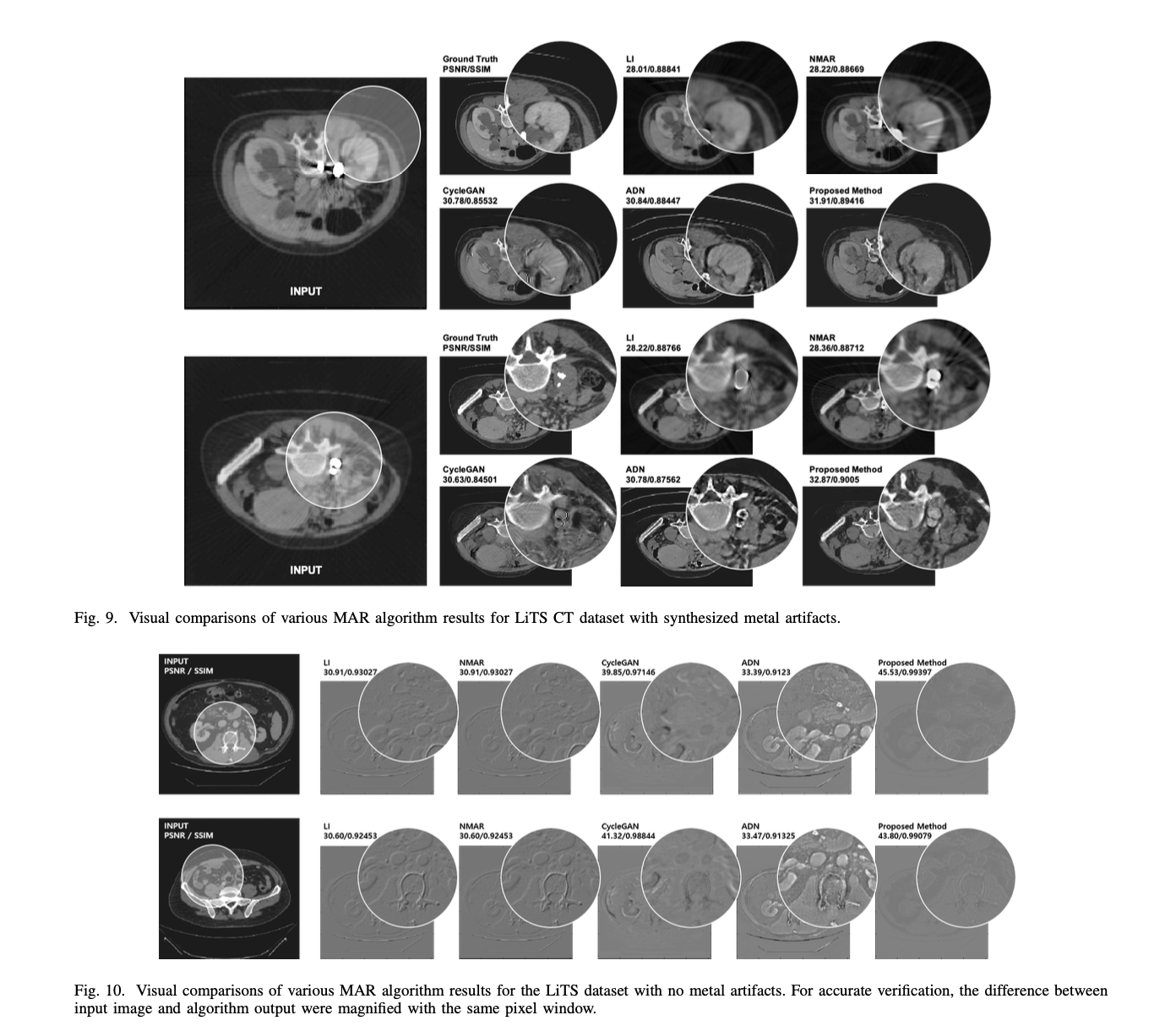
Synthetic data
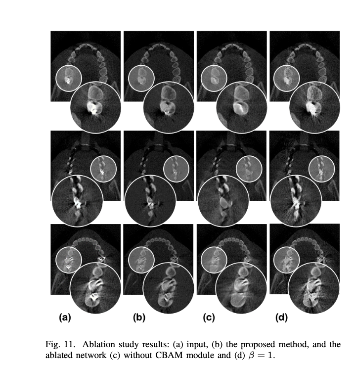
blation Study
- CycleGAN w/o CBAM
- artifacts in the background had becom fainter compared to those of the input
- real metallic objects are incorrectly removed
- Dependency on the disentanglement parameter
- $\beta$=10일때가 더 결과가 좋다
Discussion
→ novel $\beta$-cyclegan with an attention module for MAR (attention 모듈을 활용한 $\beta$-cyclegan 모델을 MAR task에 활용했다.)
local position with globally radiating artifact ⇒ CBAM to focus on important features in both spatial and channel domain (CBAM attention을 사용해 spatial/channel 모두에서 attention을 적용했다)
disentanglement parameter $\beta$ that imposes relative importance on the reconstructed artifact-free images compared to the artifact generation process (disentanglement parameter $\beta$ 가 artifact를 생성하는 네트워크(G)에 비해 artifact를 지우는 네트워크(F)에 더 비중을 가게 해준다.)
정리
MAR에서 self-supervised를 어떻게 사용하는지가 궁금해서 봤는데 역시 MAR에서 self-supervise가 supervise를 이기기는 힘든 것 같다. 성능이 많이 안 따라와줘서 조금 아쉽기도 한데, 그래도 내가 self-supervised로 문제를 풀었다면 이렇게 풀었겠구나를 그대로 따라간 것 같아 논문 하나로 내가 생각한 걸 정리할 수 있었던 것 같다. attention을 사용한 위치랑 이유가 나랑도 비슷해서 신기하기도 하고 역시 다들 비슷한 생각을 하고 있구나를 또 느낄 수 있었다..ㅋㅋ synthesized data가 너무 강력한 MAR task에서 이후에 self-supervised가 언제 그리고 어떻게 superivsed를 능가하게 될 지 궁금하다.